Not all ETFs are created equal
ETFs or Exchange Traded Funds are an investing hit of recent years. Even small investors can seamlessly open a position in a stock index or various commodities using an ETF. Previously, this was only possible by using big futures contracts that require a huge account. However, the human invention has no boundaries. More exotic ETFs, like inverse or leveraged, emerged and attracted interest from both retail and institutional traders. But let me explain first how typical (non-leveraged) ETFs work.
An ETF is basically a fund that holds some assets or performs some predefined investment strategy. Shares of this fund trade on a stock exchange like ordinary stocks. The price of these ETF shares simply tracks the net asset value of the fund, i.e. the value of all the assets (less liabilities) the fund holds. The fund charges a small fee, which is automatically deducted from the fund’s cash. But why would anyone buy ETF shares when they could buy the underlying assets directly? The main reason is time, cost savings, and simplicity. Take the SPY ETF as an example, which has a goal to replicate the S&P 500 stock index. The fund’s manager basically holds all the 500 stocks in such a ratio that corresponds to the weight of each stock in the S&P 500 index. If you would like to replicate this on your own account, it won’t be easy. First, you’d have to calculate exactly how many shares of each stock you need to buy. If you have a small account, you may find the required number of some shares to be less than one, or the rounding errors to be too significant. And even if you have a large account, calculating share allocations, and the actual process of buying 500 shares of each stock would be quite time-consuming. Not to speak of paying commission to a broker 500 times instead of once for the ETF. The expense fee a fund charges is very low. It’s just 0.1% p.a. for the SPY.
The so-called leveraged ETFs on stock indices have become very popular lately. The principle of their operation is the same as described above with one exception. A leveraged fund is able to hold positions with higher notional values than the fund’s NAV. It’s basically a margining (borrowing money to finance trades) on an institutional level.
Let’s take a look at TNA, for example. It’s a 3x leveraged ETF on the Russell 2000 index (RUT). TNA has a goal to replicate the RUT’s daily return three times. It may look like a tempting long-term investment. Instead of opening a position in Russell (through ETF IWM for example), you can open a position in TNA for just 1/3 of your intended allocation. You’d save 2/3 of your money, which can be used for other opportunities. Well, that would be nice, but there’s no free lunch. Leveraged ETFs slowly decay in value over time, which is a sort of tax we pay for the higher leverage they offer. They are really not suitable for long term holding. For instance, the TNA decays because of the compounding effect. In order to keep the leverage ratio at 300%, the fund’s portfolio manager has to rebalance positions each day. That’s because each movement in the price of the ETF changes the leverage ratio of the fund. And daily rebalancing is causing a loss of value.
I’ll demonstrate the compounding effect in a simple example. Let’s say you buy some shares for $100. The stock rises by 10% on day 1. Your investment grows in value. The next day the stock falls 10%. So one day up 10% and the next day down 10%. Maybe you think your investment is on par. Well, in fact, your stock is now worth only $99. This simple calculation proves it:
$100 * 1.10 = $110
$110 * 0.90 = $99
This effect is universal. However, the problem with leveraged ETFs is twofold. First, they don’t just hold some stocks, their goal is to replicate some leverage ratio daily, so they have to rebalance in order to do it. And second, the higher leverage ratio (2x or even 3x is common) strongly amplifies the decay in value over the longer term.
Maybe you think you can get around this by using options. Well, that’s wrong. Decay effect is propagating directly into options. Why would a market maker sell an option for $100 if he knows it’ll be worth $99 on the expiration no matter what?
By the way, pricing options on leveraged ETFs is an interesting topic. The decay of an ETF’s value strongly depends on the time to expiration, non-linearly. That just means if an ETF decays by X after 1 week, we can’t say the decay after 3 weeks will be 3*X. It won’t! It can be a wildly different (higher) value.
We can think about the decay as a tracking error, i.e. how much an ETF’s price departs from the ideal (leveraged) projection. As I said, tracking error depends on time. Besides that, it also strongly depends on realized interday volatility during the selected period. However future volatility is not known and therefore tracking error can vary substantially. This uncertainty propagates into options prices. And where there’s uncertainty, there’s opportunity!
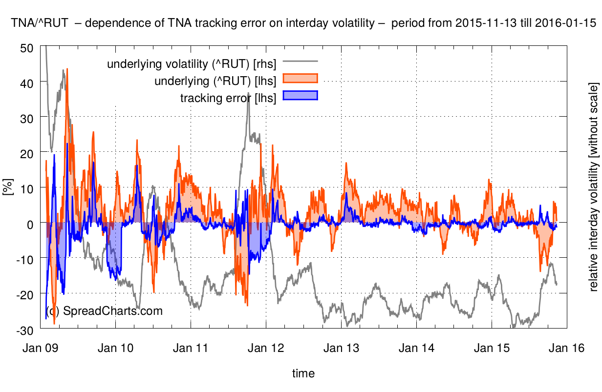
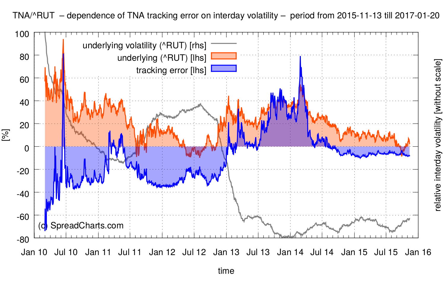
Enough theory, let’s see these effects in practice. I made a simple script, that demonstrates ETF decay. Take TNA, the triple leveraged ETF I already mentioned, as an example. The first chart shows the rolling tracking error since the inception of the ETF. The size of the rolling window over which the tracking error is calculated corresponds to the time span from today (Nov 13th, 2015) and January expiration (Jan 15th, 2016). So it’s approximately two months. The tracking error is displayed as the blue line. Negative values point to theoretical underperformance against the nominally triple long position in the underlying index (RUT). Similarly, positive values highlight periods of overperformance.
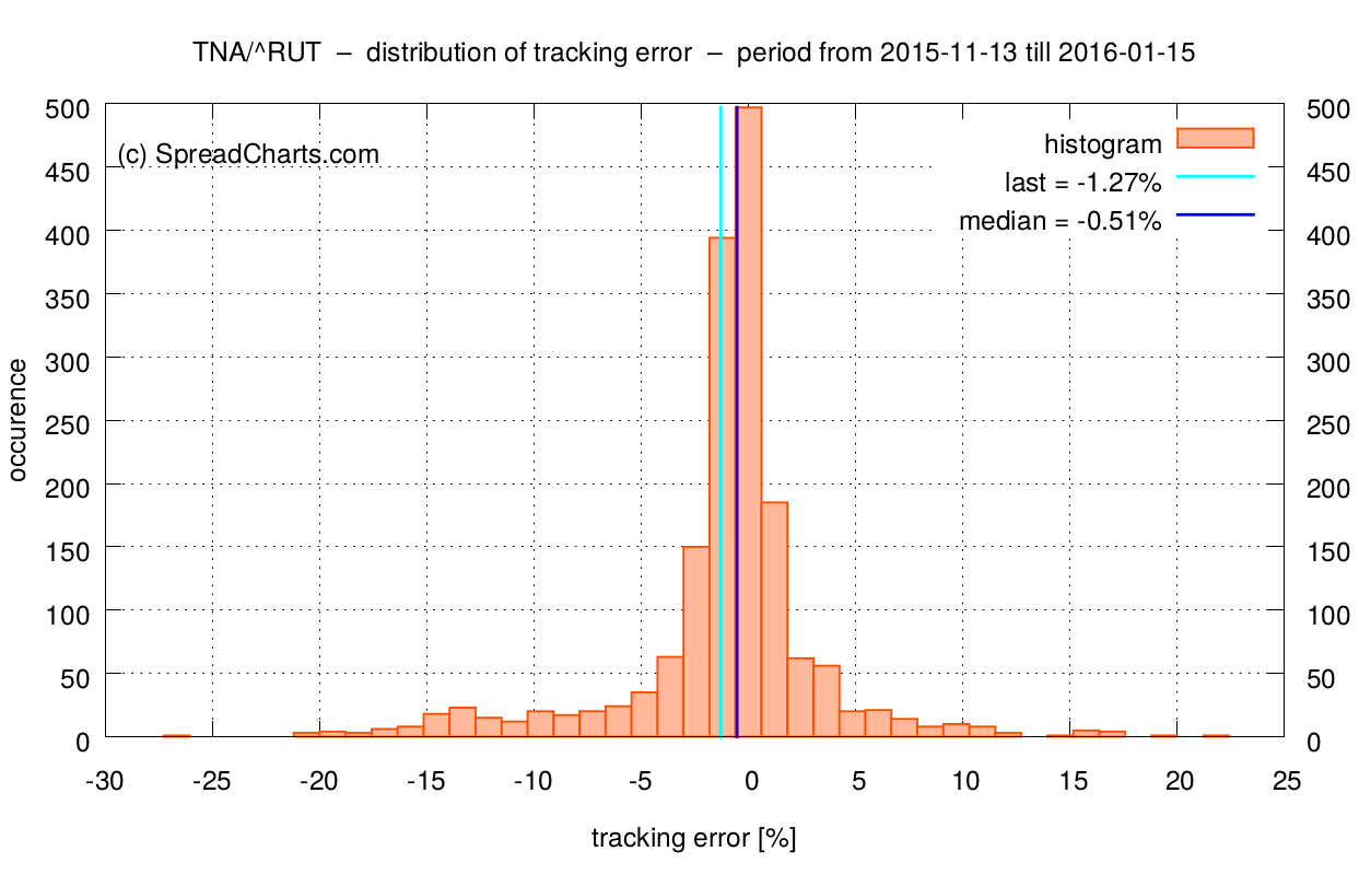
Take a look at the distribution of the tracking error. For simplicity, we can estimate the expected tracking error over 2 months as a median of the distribution, which is -0.51% in this case. What does that mean in practical terms? Assume we’d like to open an options position in TNA today (Nov 13th, 2015) using the January expiration. Then we have to expect the price of TNA to decline by 0.51% no matter how the underlying index (Russell 2000) close on the January expiration.
Well, it doesn’t sound like a big drag. Let’s see how the situation changes when we consider a more distant expiration like April 2016.
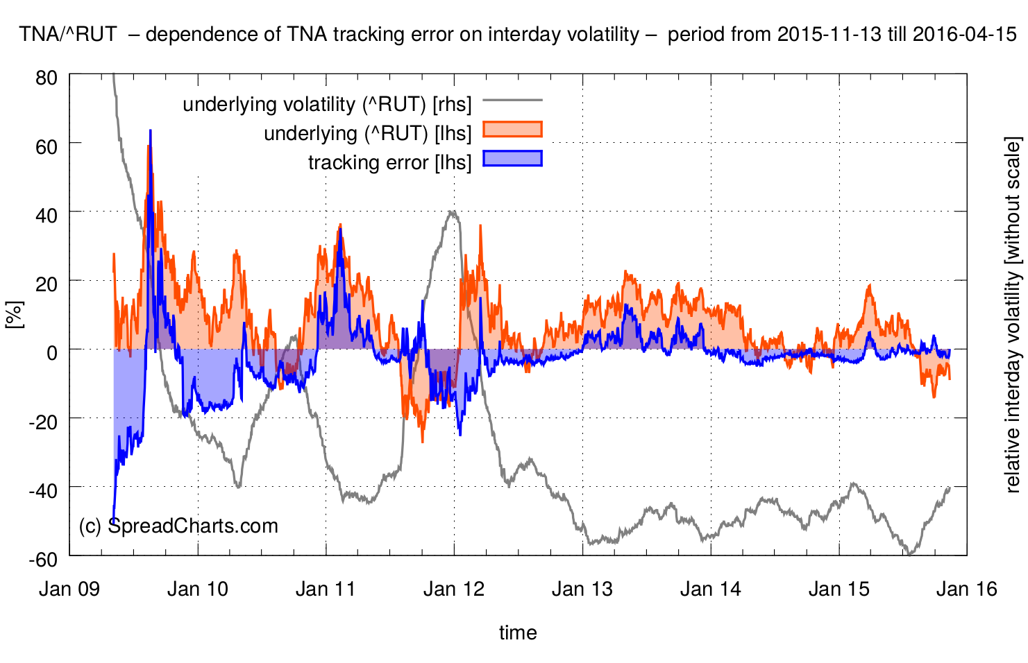
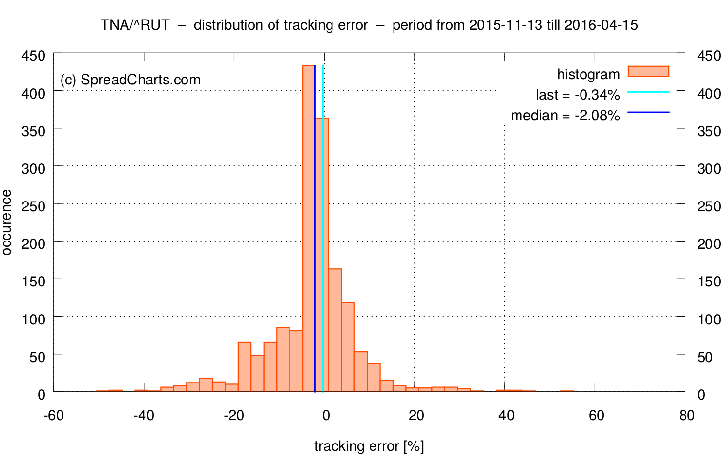
The median of the tracking error jumped to -2.08%. If you take a closer look at the first chart, you may notice the strong dependence of the tracking error on realized interday volatility over the corresponding period. This is a key observation every trader has to take into account. The tracking error is largest in situations where a portfolio manager has to rebalance a fund’s positions to a great extent in order to keep 3x leverage. And that happens in periods of high interday volatility of the underlying.
Finally, take a look at a situation where we open a position in the January 2017 expiration.
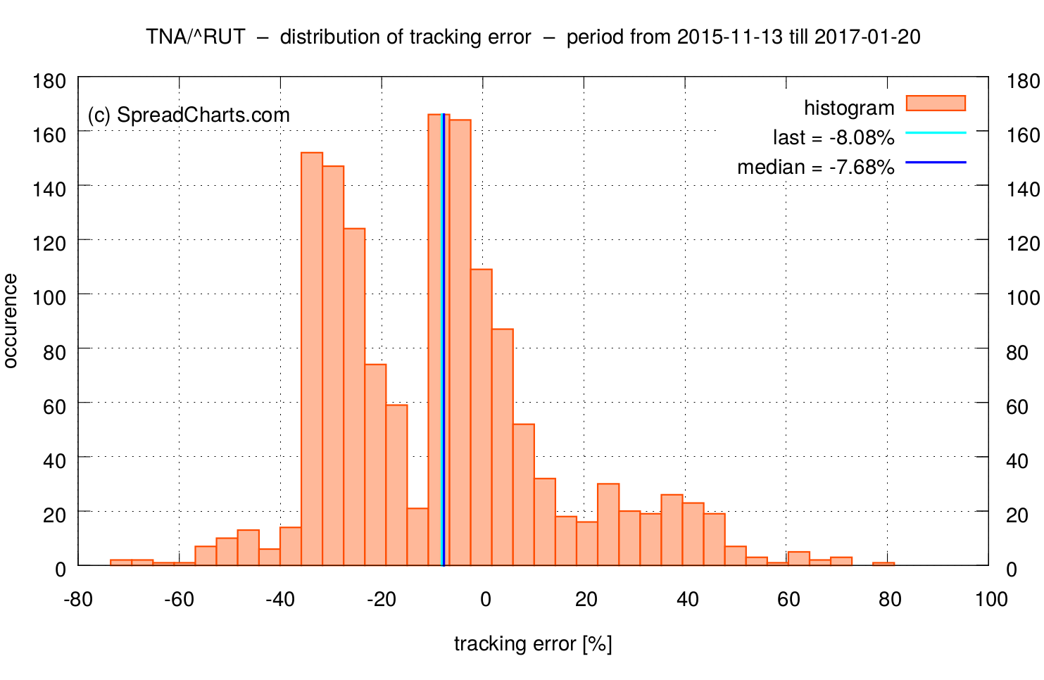
Please note the period (more than a year) is quite high compared to the history of available data. This is the reason why the distribution is so asymmetric. It will become symmetric once our dataset gets larger. Nevertheless, the median tracking error jumped to -7.68%. That’s quite a lot and it demonstrates why leveraged ETFs are unsuitable for holding over long periods of time (or for longer term option strategies).
Check out also these great articles
Why trade SGX Rubber?
Last time, we introduced the SGX data in the SpreadCharts app and briefly described the...
Read moreIntroducing commodities in Singapore
We are thrilled to announce that we have obtained a license to distribute market data...
Read moreA bunch of new data
A bunch of new data has been added to the SpreadCharts app! This includes data...
Read moreLaunching an improved model for signals
I personally consider the signals generated by our AI model to be the cornerstone of...
Read more